Monte Carlo techniques for stock price estimation

This project implements a Monte Carlo Simulation for Stock Price Prediction. This post is (heavily?) inspired from GuruFinance Insighs and by an old piece of code that I used for estimateing the benefits of some life insurance offers.

Introduction

Monte Carlo simulation is a powerful technique used in finance to model the probability of different outcomes in processes that involve random variables. In this post, I’ll walk through how to implement Monte Carlo simulations for stock price prediction using Python, using both normal distribution and Student’s t-distribution approaches.

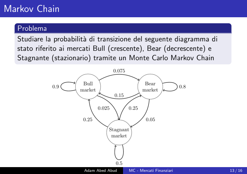
A personal note: I have always been fascinated by the use of Monte Carlo methods, especially in Finance. I was also always surprized by the fact that not a lot of people around me know about them, yet they are so powerful and widly used. In my university years I used to experiment a lot with such techniques. Here is a presentation I did more than 7 years ago in Italy:

I like Monte Carlo methods because it allow us to simulate thousands of possible future price paths for a stock, helping us understand the range of potential outcomes and their probabilities. This is particularly valuable for risk management, option pricing, and portfolio optimization. I don’t have many details about such field but I believe they must apply something similar.

Implementation

The implementation uses several Python libraries including pandas for data manipulation, yfinance for stock data retrieval, and matplotlib for visualization. Here’s how it works:

Download the historical gold data of 1 oz

# Download data
stock_gold = "GC=F"

stock = stock_gold
data = yf.download(stock, start="2018-01-01", end="2025-03-28")

adj_close = data['Close']
returns = adj_close.pct_change()

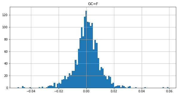
This will yield the following:

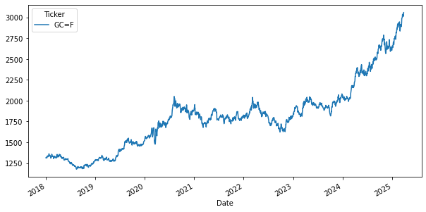
The last value as of March 28th is 3060 USD.

Monte Carlo (MC) simulation

Here comes the fun part. The MC simulation consists in simulating different outcomes for the price variation. We do 1000 simulations. For that we take the standard deviation of the historical data for the last 5 years (maybe not the best estimator?) and then we use it to get an estimation of the forecasted percentage change of price by taking a random number (normal distribution with the same std of the real std of the historical data).This is based on the assumption that stock returns follow a random walk.

We therefore can estimate the simulated price for the next year.

num_simulations = 1000
num_days = 365
daily_volatility = returns.std()

simulation_df = pd.DataFrame()
for x in range(num_simulations):
    count = 0
    price_series = [] 
    rtn = np.random.normal(0, daily_volatility)
    price = last_price * (1+rtn)
    price_series.append(price)

    for days in range(num_days):
        rtn = np.random.normal(0, daily_volatility)
        price = price_series[days] * (1+rtn)
        price_series.append(price)

    simulation_df[x] = price_series

Results of the simulation

Here are the results of the simulation

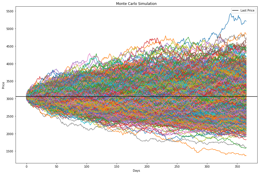
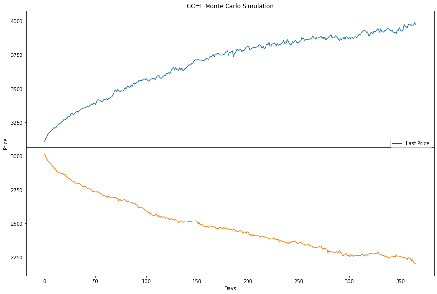
It is alsom more interesting to see them as a function of the top and bottom quantiles, in other words what is the best case scenario and the worst case scenario.

Monte Carlo Simulation with Student’s t-Distribution

While the normal distribution is commonly used, it often underestimates the probability of extreme events (fat tails) in financial markets. The Student’s t-distribution can better capture these tail risks. First, let’s fit a t-distribution to our historical returns:

# Remove NaN values from returns
returns = returns[1::]

# Fit t-distribution to returns
params = t.fit(returns)

print('degree of freedom: ', params[0])
print('mean: ', params[1])
print('standard deviation: ', params[2])

I used the t-student distribution from scipy.stats

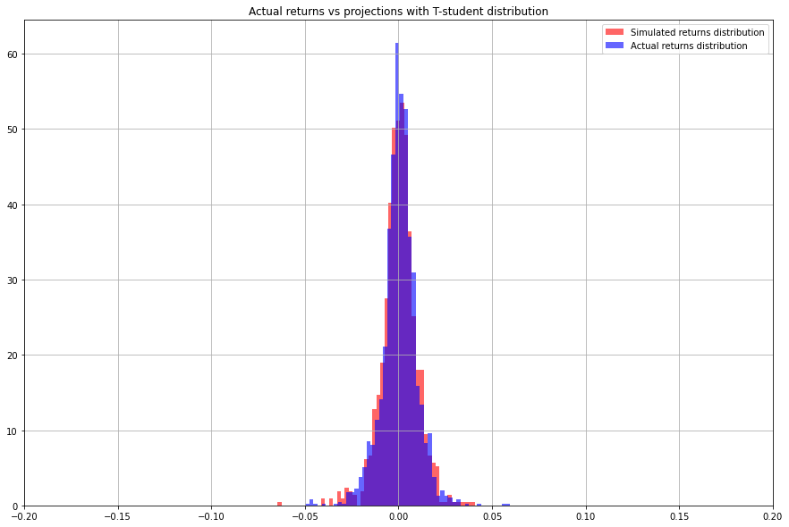
The following plot shows the distribution of the percentage change in price for gold (1 oz). Here is a plot that shows the actual distribution vs the t-student distribution:

The following step is to do the MC simulation but with parameters extracted form the t-student distribtuion:

num_simulations = 1000
num_days = 365

simulation_student_t = pd.DataFrame()

for x in range(num_simulations):
    count = 0
    price_series = [] 
    rtn = t.rvs(df=params[0], loc=params[1], scale=params[2], size=1)[0] 
    price = last_price * (1+rtn)
    price_series.append(price)
    for days in range(num_days):
        rtn = t.rvs(df=params[0], loc=params[1], scale=params[2], size=1)[0] 
        price = price_series[days] * (1+rtn)
        price_series.append(price)
    simulation_student_t[x] = price_series

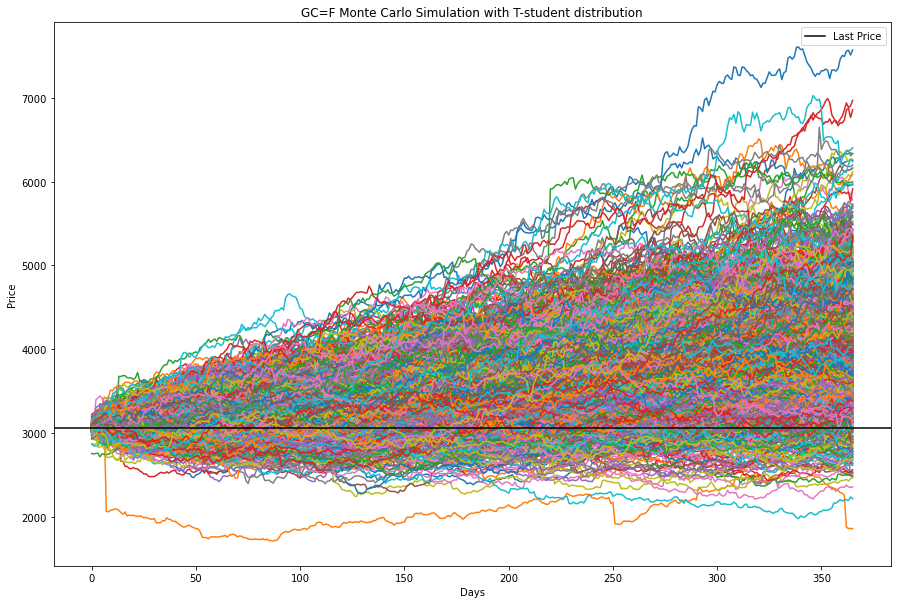
And here are the results:

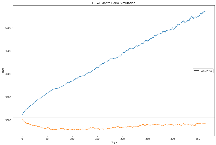
And here are the top and bottom quantiles:

The key difference between these two approaches is how they handle extreme events:

• Normal distribution: Assumes returns are symmetrically distributed around the mean with thin tails.

• Student’s t-distribution: Can better model the fat tails observed in real financial returns, capturing the higher probability of extreme events.

In practice, you’ll often notice that the t-distribution simulation shows a wider range of potential outcomes, especially in the extreme cases, which could be more realistic for risk management purposes.

Conclusion

Monte Carlo simulation is a versatile technique for modeling uncertainty in financial markets. By generating thousands of possible future price paths, we can better understand the range of potential outcomes and make more informed investment decisions. I personally use it frequently (maybe too often!).

The choice between normal and t-distribution depends on your specific needs:

• Normal distribution is simpler and works well for many applications
• T-distribution better captures extreme events and is often more appropriate for risk management

This approach can be extended to multiple assets, different time horizons, and more complex financial instruments like options and structured products.

The full code for this example can be found in this github repository with the python notebook (here).